When costs enter an allocation rule, raising the cost assumption changes both the trading bill and the trades chosen. A comparison of final returns combines those two effects.
The invented transaction lists illustrate cost accounting, with no estimate of achievable execution.
Order count and turnover answer different questions
Compare two transaction lists against the same fixed reference capital of 100,000 currency units. List A has 100 orders with executed notional of 1,000 each; List B has 20 orders with executed notional of 3,000 each. Each order is one side of a transaction.
| Invented list | Orders | Notional per order | Total traded notional | Gross turnover / initial capital | Direct cost at 5 bp per side | Cost / reference capital |
|---|---|---|---|---|---|---|
| A | 100 | 1,000 | 100,000 | 1.00× | 50 | 0.05% |
| B | 20 | 3,000 | 60,000 | 0.60× | 30 | 0.03% |
When does order count start to matter?
Keep both transaction lists fixed. Change the proportional rate, then add a fixed charge per order and compare the bills.
List A costs 50.00 and List B costs 30.00 currency units. B’s charge is 40.0% lower. The two transaction lists stay fixed.
Charge = traded notional × bp / 10,000 + order count × fixed charge. The lists stay fixed and fixed charges add to the proportional bill. Funding, minimum commissions, market impact and policy changes are not modelled. The chart keeps a fixed 0–400 scale.
Data and code
| List | Rate charge | Fixed charge | Total |
|---|---|---|---|
| A | 50.00 | 0.00 | 50.00 |
| B | 30.00 | 0.00 | 30.00 |
Interactive values (JSON) Original figure inputs Reproduction script
Static figure and caption

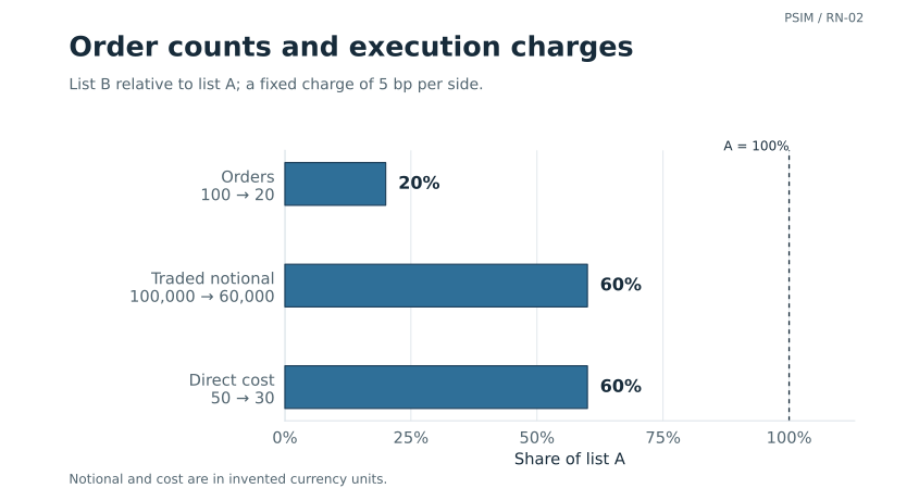
List B has 80% fewer orders and 40% less executed notional. Its proportional charge is therefore 40% lower. Funding, inventory and price evolution enter the funded replay below; these first two lists contain only orders and notionals.
For per-side notional Nj, fixed reference capital E0 and a constant cost rate c in basis points:
Direct cost = (c / 10,000) ∑j |Nj|.
Gross turnover counts every buy and sell against the fixed reference capital. Buying 1,000 and later selling 1,000 contributes 2,000. This unannualised notional ratio is not a return. Charge each order at its own rate where rates differ; minimum commissions and fixed fees add a separate dependence on order count.
State which execution effects are already included
A spread already included in the fill price must not be charged again. If the replay uses a reference price instead, it needs a fill assumption as well as a list of charges debited separately.
A blended cost assumption can combine spread, impact, fees, delay, financing and borrowing. State what it includes. Treat it as a scenario unless execution evidence supports it for the relevant market, size and order process.
Frequent input updates can leave positions unchanged for long periods. Costs follow the trades, rather than the observation frequency.
Cross the policy setting with the execution charge
The next comparison separates repricing fixed decisions from changing those decisions. Let ΠL and ΠH denote decisions generated under lower and higher assumed costs, and G(Π, c) their log growth when replayed at charge c. Within a row, keep the decisions fixed and change the charge. Within a column, keep the charge fixed and change the decisions. All four cases need the same horizon, funding and cash-flow treatment, feasible accounts and positive wealth wherever log returns are used:
| Decision process | Lower execution charge | Higher execution charge |
|---|---|---|
| Decisions generated under lower assumed cost | G(ΠL, cL) | G(ΠL, cH) |
| Decisions generated under higher assumed cost | G(ΠH, cL) | G(ΠH, cH) |
A fully specified two-trade replay
Start with 100,000 cash, no holdings and no external flows. One asset trades at 100 initially and 101 at the terminal mark. The lower-cost policy ΠL buys 500 shares at the initial mark and sells all 500 at the terminal mark. The higher-cost policy ΠH instead buys and sells 200 shares at those same prices. Treat these as two fixed decision lists; no optimization or signal estimation is performed. Each fill is complete at the stated price; an explicit fee is debited on each buy and sell. Uninvested cash earns zero; there is no spread, impact, delay, borrowing or financing charge.
The charge rates are cL = 5 bp and cH = 10 bp per side. Gross profits are 500 and 200. Total traded notionals are 100,500 and 40,200, so the four direct fees are 50.25, 100.50, 20.10 and 40.20. All purchases are affordable, all four accounts finish in cash, and wealth stays positive. Terminal wealth equals initial cash plus gross profit minus fees; G = log(terminal wealth / 100,000).
| Fixed decisions | 5 bp per side | 10 bp per side |
|---|---|---|
| ΠL: 500 shares | 100,449.75; G ≈ 0.448742% | 100,399.50; G ≈ 0.398704% |
| ΠH: 200 shares | 100,179.90; G ≈ 0.179738% | 100,159.80; G ≈ 0.159672% |
The diagonal comparison changes both the decision list and its fee rate. To separate them, first reprice the lower-cost list without changing its trades, then switch lists while holding the higher fee rate fixed. Adding and subtracting that crossed cell gives:
= [G(ΠL, cH) − G(ΠL, cL)]
+ [G(ΠH, cH) − G(ΠL, cH)].
We can reverse the order: switch policies at cL, then reprice ΠH. The first identity repriced ΠL before changing policy at cH:
= [G(ΠH, cL) − G(ΠL, cL)]
+ [G(ΠH, cH) − G(ΠH, cL)].
| Order | Cost contribution | Policy contribution | Total |
|---|---|---|---|
| Cost first, then policy | −0.050038 | −0.239031 | −0.289070 |
| Policy first, then cost | −0.020066 | −0.269004 | −0.289070 |
Both orders give the same total. Because the larger trade list is more sensitive to fees, they assign different amounts to cost and policy. The attribution is conditional on the chosen order. The download checks both identities at full precision.
Define what the replay keeps fixed
A replay needs to specify whether it holds shares, target weights or order instructions fixed. Higher debits can reduce the cash available for later orders. Rescaling those orders changes the decision list as well as its cost.
If an order becomes unaffordable, record the failure or apply a rule chosen beforehand. Retain insolvent outcomes rather than dropping them from a log-growth calculation. Decisions must also retain their original information cutoff.
The four exposure paths let us compare holdings, turnover and drawdown as well as growth. Cost and delay can be stressed together where they interact.
Reproduce the example
- Constructed transaction-list arithmetic, CSV
- Runnable examples using the Python standard library
- Arithmetic check results and scope
The downloads reproduce the order counts, traded notional, turnover, charges and the four funded replay cells, including both attribution orders.
Reproduce the figures
The figure script reproduces the charts from their published inputs. The figure data and checks record the inputs, seed and package versions.
python figures_v1.py --output-dir figuresRequires Python 3.10 or later, NumPy, SciPy and Matplotlib. Output: SVG and PNG in two layouts. Rendering varies with package versions; the supplied SVGs retain the published appearance.