A strategy can make money and still add nothing to a simpler benchmark. The test has to match the claim: positive net growth, improvement over a reference portfolio, or a contribution from one particular input.
The worked example starts from four invented p-values. It demonstrates the adjustment arithmetic; it does not estimate p-values from a return sample.
Define the contribution before choosing the test
To test an added information input, hold the position-sizing rule, execution assumptions, exposure constraints and evaluation schedule constant. Change only the input and compare the two versions of the process.
A passive benchmark brings other differences into the comparison: market exposure, volatility, holding horizon and transaction costs. Even if risk is matched in the training window, realised risk can differ during evaluation.
Choose the benchmark before seeing the results. A benchmark chosen afterwards belongs in the selection history.
Preserve the order of information
Each evaluation fold should follow its training period. Fit transformations and choose parameters using only information available before the evaluation decisions. Account for publication delays and exclude training labels whose outcomes were not yet known at that cutoff. Specify how the model will be updated before looking at the evaluation results.
The rolling-origin discussion by Hyndman and Athanasopoulos covers the training and testing order. For trading, the timing must also allow for input availability and order execution.
Once backtest results guide a redesign, that period becomes part of development. Confirmation needs later observations that did not influence the revision; until then, the result remains exploratory.
Pair the observations that answer the question
For candidate i and a specified benchmark b, define a paired log-return difference on common observation dates:
μ̂i = T−1 ∑t=1T di,t.
If the intended claim is improved mean log growth, test the one-sided hypothesis:
The example below starts with assumed p-values and works through the multiple-testing adjustment. It does not estimate the paired return effect.
Use compatible cash-flow, valuation and cost conventions for both series, with returns greater than −1. Match the observation dates on both sides. The test concerns mean incremental log growth; drawdown and comparisons with other benchmarks need their own assessment.
Return dependence and changes in the distribution affect the uncertainty estimate. Block resampling can preserve some dependence, provided the block choice and stability assumptions are justified. Holm’s correction still requires valid input p-values.
A reproducible example of multiple testing
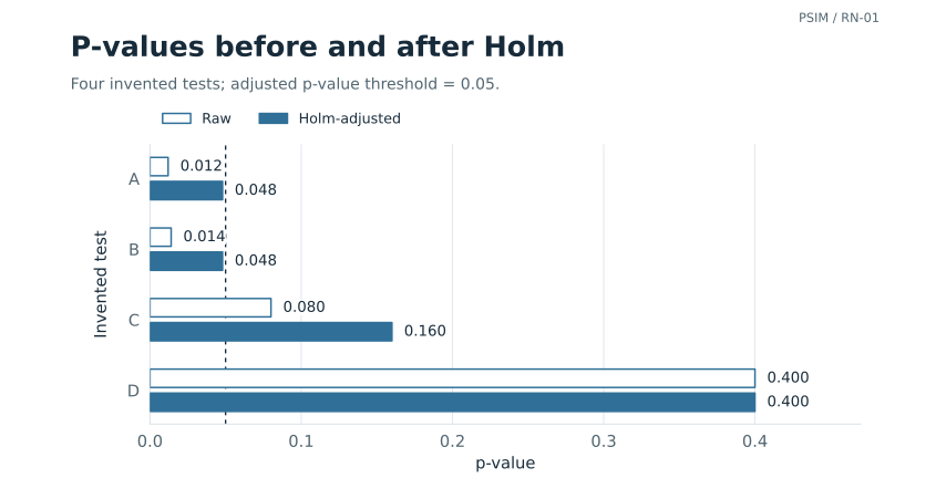
Take four hypothetical comparisons. Their assumed raw p-values are chosen to make the adjustment arithmetic visible; the labels do not correspond to instruments or strategy families.
| Invented test | Raw p-value | Holm-adjusted p-value | Reject at family-wise 5% level? |
|---|---|---|---|
| A | 0.012 | 0.048 | Yes |
| B | 0.014 | 0.048 | Yes |
| C | 0.080 | 0.160 | No |
| D | 0.400 | 0.400 | No |
How much survives the multiple-testing adjustment?
Switch between the four raw p-values and their Holm adjustments. Move the threshold to see which values clear it.
Holm-adjusted: 2 of the four invented p-values are at or below 5%. The adjustment accounts for the four-test family.
Holm takes the running maximum of (4 − rank + 1) × p, capped at 1, for these four assumed inputs. Moving α shows how the rejection decision changes; choosing it after seeing the results would add another selection choice.
Data and code
| Test | Raw p | Holm p |
|---|---|---|
| A | 0.012 | 0.048 |
| B | 0.014 | 0.048 |
| C | 0.080 | 0.160 |
| D | 0.400 | 0.400 |
Interactive values (JSON) Original figure inputs Reproduction script
Static figure and caption

For ordered raw p-values and a family of size m, the adjusted values are:
The initial products are 0.048, 0.042, 0.160 and 0.400. The second is 3 × 0.014 = 0.042, below the first product of 0.048, so the cumulative maximum raises it to 0.048. The table shows the final adjusted values. The statsmodels documentation identifies Holm as a step-down Bonferroni procedure.
Holm controls the probability of at least one false rejection in the specified family, provided each null p-value is valid for that testing procedure. It does not require independence between the tests. The R documentation describes this family-wise control.
Applying Holm only to the survivors of a search does not generally correct for that search. A frozen shortlist can be tested on separate confirmation data, or an inference procedure can account for selection. For a family fixed beforehand, correcting all its valid tests can cover that family. Adaptive searches need further justification. An adjusted p-value is not the probability that a strategy is useful.
Separate statistical and economic conclusions
Report the size of the improvement alongside its uncertainty, trading costs, turnover and variation across evaluation periods. A statistically detectable effect may be too small to cover costs; a large estimate may still be too uncertain to rely on.
Count hypotheses separately from simulation runs. Several stress settings for the same comparison are not independent discoveries, especially when they share data, controls and training histories.
Reproduce the example
- Invented p-values and adjusted values, CSV
- Runnable examples using the Python standard library
- Arithmetic check results and scope
The script reproduces the Holm adjustment from the four printed p-values. It does not estimate them or establish their validity. Running it requires only Python 3.9 or later; python reproduce_examples.py --output-dir examples also writes the CSV and check files.
Reproduce the figures
The figure script reproduces the charts from their published inputs. The figure data and checks record the inputs, seed and package versions.
python figures_v1.py --output-dir figuresRequires Python 3.10 or later, NumPy, SciPy and Matplotlib. Output: SVG and PNG in two layouts. Rendering varies with package versions; the supplied SVGs retain the published appearance.