Take two loss models. Both have a mean of zero and a standard deviation of one. In the first, the average loss in the worst 1% of outcomes is 2.67. In the second, it is 3.45. A variance report gives them the same headline number.
The previous note used covariance to solve portfolio problems across 10,000 equities. To understand large losses and their tendency to arrive together, we need more of the distribution.
Every input is invented. Losses are additive shocks in arbitrary units over one unspecified horizon; a negative loss means a gain. These unbounded shocks are not simple returns on limited-liability equities and should not be compounded into stock prices.
The first examples measure losses for fixed weights. We then let the risk model choose the weights; a higher expected shortfall need not change the allocation.
1. The same covariance can describe different risks
For portfolio loss L = w⊤X, with asset loss shocks X, variance is w⊤Σw. Calculating the probability of a very large loss also requires a joint distribution. [1]
We can make the distinction exact. Choose a positive-definite matrix Σ and a factor B satisfying BB⊤ = Σ. Let Z be a vector of independent standard normals. Independently draw U from a chi-squared distribution with ν degrees of freedom. Compare:
Xt = √[(ν − 2)/U] BZ, ν > 2.
The second construction is a variance-normalised multivariate Student-t. The same random multiplier applies to every component, so a small U enlarges all the Gaussian shocks together. This normal-mixture representation also underlies the t copula. [2] Since E[1/U] = 1/(ν − 2), the squared multiplier has expectation one. Both vectors therefore have mean zero and covariance Σ.
The restriction ν > 2 matters: at or below that boundary, this finite-covariance comparison is unavailable. A standard univariate Student-t has variance ν/(ν − 2), so multiplying it by √[(ν − 2)/ν] gives variance one. [3] We use ν = 5.
| Loss model | Mean | Variance | 99% VaR | 99% ES |
|---|---|---|---|---|
| Gaussian | 0 | 1 | 2.3263 | 2.6652 |
| Student-t, 5 degrees of freedom | 0 | 1 | 2.6065 | 3.4488 |
Same variance. How different can the tail be?
Change the Student-t tail thickness and the confidence level. Compare the threshold loss with the average loss beyond it.
At 99% confidence, Gaussian expected shortfall is 2.67 and Student-t expected shortfall is 3.45. Both models still have mean zero and variance one. Values are arbitrary additive loss units.
Analytic distributions, both with mean 0 and variance 1. Student-t is scaled by √[(ν − 2)/ν], with ν > 2. Dots mark VaR at the selected exceedance probability; expected shortfall averages the tail beyond it. The probability axis is logarithmic and ends at 0.001%; the distribution continues. Arbitrary additive loss units are not equity simple returns.
Data and code
| Loss model | VaR | Expected shortfall |
|---|---|---|
| Gaussian | 2.3263 | 2.6652 |
| Student-t (5) | 2.6065 | 3.4488 |
Interactive values (JSON) Original figure inputs Reproduction script
Static figure and caption

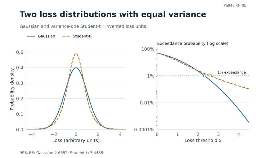
The Student-t expected shortfall is 29.4% higher. The download checks the analytic result by separately integrating the tail density.
Both marginal tails and dependence change in this comparison. Isolating a copula effect would require holding the marginals fixed. The covariance match is at the population level; finite simulated samples will differ.
2. How often do the large losses arrive together?
A copula separates marginal distributions from their dependence. For continuous marginals F1 and F2, write the joint distribution as C(F1(x), F2(y)). The transformed variables are uniform on [0, 1]; C describes their joint behaviour. [1]
For a risk question, we can look directly at a conditional probability: given that one loss exceeds its own 99th percentile, how often does the other exceed its 99th percentile too? Use each model's own quantiles so that the marginal exceedance probabilities agree.
λU = limu→1 χ(u), when the limit exists.
The limit λU is upper-tail dependence. With −1 < ρ < 1, a Gaussian copula has λU = 0. A t copula has:
Here Tν+1 is the Student-t cumulative distribution function. At ν = 5 and ρ = 0.5, the coefficient is 0.207031. [2] That is a limiting conditional probability, not the probability of a market crash.
| Marginal quantile | Gaussian | Student-t, 5 degrees of freedom |
|---|---|---|
| 95% | 24.38% | 32.13% |
| 99% | 12.94% | 25.94% |
| 99.9% | 5.43% | 22.62% |
The table evaluates χ(u) by numerical integration at correlation 0.5. It shows how conditional exceedance changes as the marginal threshold moves further into the tail.
The Gaussian entries remain positive at finite thresholds despite a zero asymptotic coefficient. The Student-t limit also differs from its 99th-percentile result. Both models are symmetric between upper and lower tails; market losses may call for an asymmetric model.
3. A threshold and the losses beyond it
For a loss L and 0 < α < 1, value-at-risk at level α is the left quantile:
VaR locates a boundary. It does not say how far losses extend beyond it. For an integrable loss, expected shortfall averages the upper quantiles:
This definition also handles discrete distributions. With a continuous loss distribution at the threshold, it agrees with the conditional mean above VaR. When probability is concentrated exactly at VaR, a conditional mean can give the wrong answer. [4]
Consider an invented loss of zero with probability 99%, and 10 with probability 1%. Its 97.5% VaR is zero. The worst 2.5% comprises the entire 1% mass at 10 plus 1.5% at zero, giving:
Conditioning on L ≥ 0 gives 0.1; conditioning on L > 0 gives 10. Neither gives 4. The same issue arises with finite scenario sets, which are discrete even when drawn from a continuous distribution.
For equally weighted scenarios, sort the losses from largest to smallest and take exactly M(1 − α) observations' worth of probability. If that number is fractional, include only the needed fraction of the boundary observation. The definition is about probability mass, not an arbitrary rule for rounding a tail count. [5]
Expected shortfall also respects diversification in the sense of subadditivity: ES(L1 + L2) ≤ ES(L1) + ES(L2). Together with monotonicity, positive homogeneity and translation by a certain loss, this makes it a coherent risk measure. [4] The coherence framework gives consistency requirements for a risk measure. [6] It does not certify the probabilities supplied to that measure.
4. Turn expected shortfall into an optimization problem
Sorting losses works for a fixed portfolio. Searching over portfolio weights becomes easier with the Rockafellar–Uryasev representation:
(x)+ = max(x, 0).
The threshold η is a decision variable. For a continuous distribution, differentiating with respect to η gives 1 − P(L > η)/(1 − α); the minimum occurs at a quantile. The representation remains valid at atoms, where derivatives are replaced by subgradients. We use CVaR as a synonym for this definition of ES. [7]
Let ℓj contain asset losses in scenario j. Portfolio loss is ℓj⊤w. With M equally weighted scenarios and an upper weight bound c, introduce slack variables uj:
subject to uj ≥ ℓj⊤w − η, uj ≥ 0,
1⊤w = 1, 0 ≤ wi ≤ c.
At the optimum, each slack records the positive excess above η. With affine losses and linear constraints, the whole problem is a linear program. Unequal scenario probabilities replace 1/M with pj. [7]
The implementation leaves η unrestricted because the loss quantile can be negative. It checks weights, constraint residuals and the primal–dual gap using the solution and marginal values from SciPy’s HiGHS interface. [8]
When a new risk measure leaves the portfolio unchanged
The common multiplier in the first model family matters for allocation. Every fixed nonzero portfolio is a linear projection with the same standardised distribution, scaled by √(w⊤Σw). For either zero-mean model, at α = 0.99:
k = 2.665214 for the Gaussian model;
k = 3.448837 for the variance-normalised t5 model.
The constant is positive, so minimizing either population ES is the same as minimizing portfolio volatility. Under matching constraints, both select the minimum-variance portfolio despite reporting different risk levels. This relies on zero means, linear losses and a fixed common distributional family. The stress model below changes that structure by giving assets different exposures to one loss event.
5. A stress model that changes the allocation
We now construct three invented assets. They share a small normal shock and an occasional positive loss shock, but their exposure to the latter differs. Let Z0, ZA, ZB and ZC be independent standard normals. Independently, let I be one with probability p = 0.04 and zero otherwise:
XB = 0.20 Z0 + 0.95 ZB
XC = 0.20 Z0 + 0.65 ZC + 1.5(I − p).
Subtracting p centres the event term, so each asset's population mean loss is zero. Asset A has relatively little ordinary noise and the largest event exposure. B has more ordinary noise and no event exposure. C sits between them. The 4% event weight is invented; it is not an estimated probability of a market crash.
The covariance is known from the construction. With s = (0.35, 0.95, 0.65) and j = (4, 0, 1.5):
We compare equal weights, the minimum-variance portfolio from this population covariance, and minimum sample ES from 20,000 generated scenarios: at 99% ES this supplies 200 scenarios’ worth of tail mass. All use a fully invested, long-only budget with an invented 80% per-asset cap. The cap is nonbinding here: no displayed allocation exceeds about 55%, so it does not change these solutions. The unconstrained budget-only minimum-variance weights happen to satisfy those bounds, so they also solve that constrained variance problem.
| Portfolio | Asset A | Asset B | Asset C |
|---|---|---|---|
| Equal weight | 33.33% | 33.33% | 33.33% |
| Minimum variance | 24.39% | 31.24% | 44.36% |
| Minimum sample ES | 0.00% | 45.50% | 54.50% |
The sample-ES solution drops A and puts more weight in B and C. Population standard deviation rises, while the average loss in the worst 1% falls under this mixture.
| Portfolio | Population standard deviation | Population 99% ES | Fresh-sample 99% ES |
|---|---|---|---|
| Equal weight | 0.5744 | 2.3296 | 2.3381 |
| Minimum variance | 0.5674 | 2.1699 | 2.1795 |
| Minimum sample ES | 0.6148 | 1.7194 | 1.7286 |
“Population ES” is calculated from the known model after the weights are fixed. Conditional on I, each portfolio loss is normal, so its unconditional distribution is a two-normal mixture. The code solves its quantile equation and integrates each normal component's tail analytically. A separate set of 100,000 fresh draws provides the evaluation column: 1,000 scenarios’ worth of tail mass at 99% ES. The training and evaluation random seeds are different.
Training ES is 1.6829, below the population value of 1.7194. Optimizing a finite sample can make its estimated risk optimistic. The fresh-sample column measures integration error on new draws from the same invented model, rather than validating it against market observations.
Sensitivity: change the event probability
This separate comparison recalculates both minimum variance and minimum population 99% ES at event probabilities of 1%, 4% and 10%. The ordinary shock scales (0.20; 0.35, 0.95, 0.65), event loadings (4, 0, 1.5), fully invested long-only budget and 80% cap stay fixed. The event term is re-centred as I − p at each probability, so mean losses remain zero. The cap is nonbinding in all six solutions.
| Event probability | Objective | Asset A | Asset B | Asset C | Population SD | Population 99% ES |
|---|---|---|---|---|---|---|
| 1% | Minimum variance | 51.98% | 18.14% | 29.88% | 0.4514 | 2.5027 |
| 1% | Minimum population ES | 8.72% | 38.69% | 52.60% | 0.5529 | 1.5739 |
| 4% | Minimum variance | 24.39% | 31.24% | 44.36% | 0.5674 | 2.1699 |
| 4% | Minimum population ES | 0.00% | 45.10% | 54.90% | 0.6140 | 1.7194 |
| 10% | Minimum variance | 4.55% | 40.66% | 54.78% | 0.6380 | 1.9044 |
| 10% | Minimum population ES | 0.00% | 50.10% | 49.90% | 0.6497 | 1.8197 |
At 1%, minimum population ES keeps 8.72% in A; at 4% and 10%, it drops A. Minimum-variance weights also move because changing the event probability changes covariance. Each row uses its own probability, so the comparisons change both the model and the selected weights.
The ES calculation minimizes the exact two-normal-mixture expectation η + E[(L − η)+]/0.01 using its analytic gradient. It uses no scenario sample. At 4%, its B/C weights are 45.10%/54.90%; Exhibit 3's sample solution remains 45.50%/54.50%. The separate sensitivity script and full-precision results include budget and bound checks, convex optimality residuals, independent starts and numerical tail integration checks.
6. Evaluate fixed portfolios across 10,000 equities
For 10,000 constructed assets, we evaluate three fixed portfolios. The CVaR optimization above remains a three-asset problem.
For this workload, the large object would be the asset-level scenario array. A 10,000 × 10,000 float64 covariance takes 800 MB; 100,000 scenarios for those 10,000 assets take 8,000,000,000 bytes: 8 GB, before temporary arrays and solver workspace. We can avoid that array when evaluating a few fixed linear portfolios.
Return to the factor covariance Σ = AA⊤ + D, with D diagonal and positive. Put P fixed portfolio vectors into the columns of an N × P matrix W. Their joint loss covariance is:
= (A⊤W)⊤(A⊤W) + W⊤DW.
If H is positive definite, factor it as CC⊤. For the common-scale Student-t model, draw a P-dimensional standard normal z and an independent U ∼ χ²5. The vector √(3/U)Cz has exactly the joint distribution of those P portfolio losses under the assumed model. We never need to materialise each asset shock. A singular H would need a suitable positive-semidefinite factorisation instead.
Forming H takes O(NKP + KP² + NP²) work, with K factors and P fixed portfolios. At K ≤ N, this simplifies to O(NKP + NP²). Factoring H costs O(P³); each later scenario costs O(P²). A single fixed portfolio reduces to one loss scalar.
The download constructs 10,000 assets and 50 factors, then evaluates three fixed portfolios: equal weight across all assets, equal weight across 1,000 assets with lower common-factor exposure, and weights proportional to a linear sequence from 1 to 2. It generates 100,000 joint portfolio scenarios in batches of 2,000.
| Portfolio | Analytic 99% ES | Simulated 99% ES |
|---|---|---|
| All 10,000, equal weight | 0.569113 | 0.570343 |
| Lower common exposure, 1,000 equal weights | 0.152043 | 0.152035 |
| All 10,000, linear tilt | 0.620853 | 0.622191 |
The subset contains the 1,000 lowest loadings on the constructed common factor, stored first in the array. Its lower risk follows from those assigned exposures; array order has no economic meaning. The scenario estimates agree with analytic Student-t ES within the reported sampling diagnostics.
The factor matrix and diagonal occupy 4.08 MB, the three weight vectors 0.24 MB, and retained portfolio losses 2.4 MB. A 2,000 × 3 loss block is 48 KB. These payload sizes exclude temporary arrays and other peak-memory costs.
Evaluation and optimization are different workloads
Linear projection preserves the distributional family for these fixed portfolios. The analytic ES therefore gives a check on the simulation. Nonlinear payoffs, changing holdings or asset-level constraints can instead require the underlying scenarios to be retained or regenerated.
The general scenario LP has N weights, one threshold, M slack variables and M loss constraints. At 10,000 weights and 100,000 scenarios, that is 110,001 variables before other constraints. A dense loss-constraint block contains roughly a billion coefficients, even if the solver uses sparse storage elsewhere.
Batching controls memory for evaluation at fixed weights. Large optimizations need additional structure, scenario reduction, generated constraints or a solver that works with the relevant operators. Scenario reduction also needs checks on the resulting approximation.
7. The model still decides what counts as a bad outcome
If a dependence model omits a shared loss event, an optimizer may concentrate in the assets whose risk is most understated. Correctly solving that optimization preserves the omission.
With 252 observations, the upper 1% contains only 2.52 observations’ worth of sample mass. Fitting a smooth density and drawing 100,000 scenarios can improve integration accuracy, but the tail estimate still rests on those 252 observations.
Vary the tail parameter, common-shock weight, dependence structure and portfolio constraints, then assess fixed weights under other models. In a market study, fit and choose the portfolio before its evaluation period and use later observations to assess it.
A one-period loss measure leaves out the drawdown path, intermediate cash needs and liquidation time. Financing, impact, changing liquidity and instrument payoffs need to be specified for the application. The notes on execution costs and linked drawdown work through those parts of the accounting.
8. Reproduce the calculations
The Python download reproduces the original numerical exhibits. The separate sensitivity download above reproduces the event-probability table. The results file records inputs, seeds, runtime versions, solver residuals and all 35 checks. It requires NumPy and SciPy:
python -m pip install numpy==2.3.5 scipy==1.16.3 matplotlib==3.10.7

python tail_risk_v3.py
The script prints JSON and reads no input files or network resources. It checks the density integral, probability mass at a quantile, a fractional empirical tail, the LP's primal and dual conditions, and the projected covariance against a separate dense calculation on 128 assets. Fresh simulation estimates are compared with the known model values.
Sampling diagnostics use the standard deviation of η + (L − η)+/(1 − α), divided by √M, at the known population quantile η. They describe integration error conditional on these invented models. The finite-draw checks are diagnostics, not coverage proofs. No market parameter uncertainty is included.
Tested with Python 3.13.9, NumPy 2.3.5 and SciPy 1.16.3. Last floating-point digits and solver choices can vary across versions. Tables round the stored calculations; the reproducible file retains full precision.
Version 1.3: the download manifest records the exact SHA-256 of each linked code and data file for this revision.
Reproduce the figures
The figure script reproduces the charts from their published inputs. The figure data and checks record the inputs, seed and package versions.
python figures_v1.py --output-dir figuresRequires Python 3.10 or later, NumPy, SciPy and Matplotlib. Output: SVG and PNG in two layouts. Rendering varies with package versions; the supplied SVGs retain the published appearance.
References
- Paul Embrechts, Alexander McNeil and Daniel Straumann (1998). Correlation and Dependency in Risk Management: Properties and Pitfalls. Author-hosted working paper, November 1998. Correlation, copulas and tail dependence.
- Stefano Demarta and Alexander J. McNeil (2005). The t Copula and Related Copulas. International Statistical Review 73(1), 111–129. Normal mixtures and t-copula dependence.
- SciPy documentation. Student's t distribution. Density, distribution and moment calculations; accessed 8 September 2026.
- Carlo Acerbi and Dirk Tasche (2002). On the Coherence of Expected Shortfall. Journal of Banking & Finance 26(7), 1487–1503. Quantile definitions, discontinuities and coherence.
- Carlo Acerbi and Dirk Tasche (2001). Expected Shortfall: A Natural Coherent Alternative to Value at Risk. arXiv working paper. Sample tails and alternative representations.
- Philippe Artzner, Freddy Delbaen, Jean-Marc Eber and David Heath (1999). Coherent Measures of Risk. Mathematical Finance 9(3), 203–228; linked author version dated July 1998. Consistency properties of risk measures.
- R. Tyrrell Rockafellar and Stanislav Uryasev (2002). Conditional Value-at-Risk for General Loss Distributions. Journal of Banking & Finance 26(7), 1443–1471; linked author version dated November 2001. CVaR representation and optimization with discrete scenarios.
- SciPy documentation. Linear programming with linprog. HiGHS interface, bounds and solution diagnostics; accessed 8 September 2026.