Geometric Brownian motion gives a useful route from Itô’s lemma to a simulator and an option price. The same machinery then leads to joint price shocks, portfolio risk and optimization across 10,000 equities, without storing a dense covariance matrix.
All numerical inputs are invented. The examples illustrate public mathematical methods.
1. A model for proportional price changes
Let St be a positive asset price and Wt standard Brownian motion: its non-overlapping increments are independent, and an increment over length Δt is normal with mean zero and variance Δt. Geometric Brownian motion (GBM) specifies:
Here μ is the instantaneous expected proportional return per year; σ is volatility per square root of a year. We use constant coefficients, σ > 0, and time in years. A one-year horizon therefore has T = 1. Brownian uncertainty scales with √Δt, while the drift contribution scales with Δt. Mixing those units produces an incorrect simulator.
GBM models proportional shocks with independent Gaussian log increments. Positive prices and a tractable solution make it a useful reference model; the increment assumptions still need checking against observations. [1]
2. Why the ordinary chain rule needs another term
For a smooth function f(t, S), once differentiable in time and twice in price, Itô’s lemma gives the following continuous-diffusion identity. Subscripts on f denote partial derivatives.
The extra term comes from quadratic variation. On successively finer partitions, the sum of squared Brownian increments converges to elapsed time. The shorthand (dW)² = dt expresses that limiting property; it is not an equality between individual finite random increments. This is why second-order curvature survives in the stochastic chain rule. [2]
Apply the formula to f(S) = log S. Since fS = 1/S and fSS = −1/S², direct substitution yields:
ST = S0 exp[(μ − ½σ²)T + σWT].
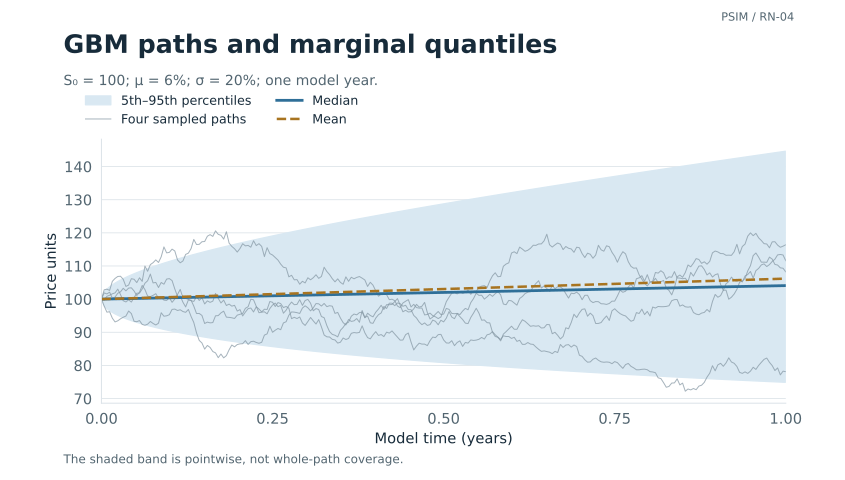
The −½σ² term distinguishes the expected log return from the proportional drift. With invented values S0 = 100, μ = 6%, σ = 20% and T = 1, the expected log return is 4%. The following quantities are calculated directly from the resulting lognormal distribution:
| Quantity | Formula | Value |
|---|---|---|
| Mean terminal price | S0 exp(μT) | 106.1837 |
| Median terminal price | S0 exp[(μ − ½σ²)T] | 104.0811 |
| 5th percentile | S0 exp[(μ − ½σ²)T + σ√T Φ−1(0.05)] | 74.9034 |
| 95th percentile | S0 exp[(μ − ½σ²)T + σ√T Φ−1(0.95)] | 144.6245 |
Φ is the standard normal cumulative distribution function. Large positive outcomes pull the mean above the median. The percentile interval describes terminal prices under the specified model, rather than path minima or uncertainty about a calibrated market forecast.
More volatility, the same Brownian draws
Change volatility while keeping drift and the four random paths fixed. Move through the model year to inspect its distribution at a chosen time.
At step 252 of 252 and volatility 20%, the model mean is 106.18 and median 104.08. The same four Brownian draws are reused. The band covers 90% at this time, not 90% of entire paths.
S₀ = 100; physical drift μ = 6%; 252 steps over one model year. Uses the same four seeded Brownian draws as the published figure (seed 20260909). S(t) = S₀ exp[(μ − σ²/2)t + σW(t)]. The mean is independent of σ; the median is not. Faint coloured lines are illustrative paths. The band is pointwise, not a path-survival band. The price axis stays fixed across settings.
Data and code
| At selected step | Price |
|---|---|
| Illustrative path 1 | 116.41 |
| Illustrative path 2 | 108.21 |
| Illustrative path 3 | 78.12 |
| Illustrative path 4 | 111.57 |
| Mean | 106.18 |
| Median | 104.08 |
| 5th percentile | 74.90 |
| 95th percentile | 144.62 |
Interactive values (JSON) Original figure inputs Reproduction script
Static figure and caption

3. Algorithm one: simulate the exact transition
The lognormal solution also gives a simulation step. For constant-coefficient GBM, draw an independent standard normal Zn at each step and use the exact transition:
The letter a makes the drift choice explicit. Use μ for a physical scenario model. Use r for the zero-dividend pricing model in the next section. In Python, the mathematical core is:
def gbm_step(s, drift, sigma, dt, z):

    return s * exp((drift - 0.5*sigma**2)*dt

                   + sigma*sqrt(dt)*z)
The complete download includes input checks and imports. The transition is exact in distribution at the sampled times, subject to floating-point arithmetic. Barriers, running maxima and continuously monitored stops also depend on what happens between those times.
Euler–Maruyama instead uses Sn+1 = Sn(1 + aΔt + σ√Δt Zn). Its normal shock can make the multiplier negative. For SDEs without a tractable transition, numerical methods are necessary, and convergence and stability become separate validation questions. [3]
4. From Itô’s lemma to an option price
To turn the price model into a valuation, consider a European call with payoff max(ST − K, 0). Assume no dividends, constant interest rate r and volatility σ, continuous trading, unrestricted borrowing and shorting at the model terms, and no transaction costs. Let its value before expiry be V(t, S).
A self-financing replicating portfolio holds Δ = VS shares and cash B = V − ΔS. Its gain is dV = Δ dS + rB dt. Matching this gain to Itô’s formula cancels the diffusion term and the μ terms, leaving:
V(T, S) = max(S − K, 0).
The cash account funds changes in the share holding; ΔS is not a constant-share product that can be differentiated while ignoring rebalancing flows. That self-financing condition is essential to the replication argument. [1]
Under these assumptions, the same price can be written as a discounted expected payoff under the pricing measure Q, where the stock drift is r:
C = S Φ(d1) − K e−rτ Φ(d2)
d1 = [log(S/K) + (r + ½σ²)τ] / (σ√τ)
d2 = d1 − σ√τ, τ = T − t.
The expectation and PDE are connected by the Feynman–Kac representation, under the appropriate regularity and integrability conditions. For a European call, the expectation has the Black–Scholes closed form shown above. [4] [5]
The physical model uses μ to describe price behaviour. Replication prices the payoff under a measure with drift r, regardless of investors’ expected return. The 6% physical drift from Exhibit 1 therefore drops out of the call price.
5. Algorithm two: price by Monte Carlo
The closed form gives a benchmark for the simulation. Set S0 = K = 100, r = 3%, σ = 20% and T = 1, still with no dividends. The call value is 9.4134 price units. Estimate it by sampling terminal prices with drift r, evaluating the payoff, discounting once and averaging.
The implementation uses antithetic variates. For each independent normal draw Zi, calculate one payoff at +Zi and another at −Zi. The pair average Yi is one observation:
Ĉ = (1/M) Σi=1…M Yi, SE = sY / √M.
The two members of a pair are dependent. Computing a standard error as though all 2M payoffs were independent would be incorrect. Here sY is the sample standard deviation of the M pair averages, using denominator M − 1.
| Independent pairs | Payoff evaluations | Estimate | Standard error | Approx. 95% interval |
|---|---|---|---|---|
| 1,000 | 2,000 | 9.1559 | 0.2298 | 8.7054–9.6063 |
| 10,000 | 20,000 | 9.4780 | 0.0748 | 9.3314–9.6247 |
| 100,000 | 200,000 | 9.4086 | 0.0235 | 9.3627–9.4546 |
All rows use nested prefixes of one stream with seed 20260908; they are not independent experiments. The approximate 95% intervals are Ĉ ± 1.96 SE, based on the central limit theorem. Sampling error need not fall monotonically in a single run. These intervals describe integration uncertainty conditional on the model and inputs. They exclude parameter uncertainty, transaction costs and model misspecification.
The discounted stock mean provides a second check on drift and discounting: 99.9980, with standard error 0.0089, against a theoretical value of 100. Both payoffs use terminal draws directly and have no time-grid bias.
6. Sensitivities become hedge calculations
Differentiating the call formula gives delta and gamma, with φ the standard normal density:
For the invented contract, Δ = 0.598706 and Γ = 0.0193334 per price unit. A short position in one option on one share has its first-order stock exposure offset by holding about 0.598706 shares at this instant. A real contract multiplier scales that amount. As price and time change, so does the required holding.
For a small price change h, with time and volatility fixed, ΔC ≈ Δh + ½Γh². The code checks both derivatives using central price differences with h = 0.01. Elapsed time, volatility changes and financing add other terms to a hedge calculation.
A discrete hedge trades the change in delta through the cash account, including fees and funding. Its residual error depends on the path and trading schedule. Jumps can break the local diffusion approximation, so a hedge test also needs explicit cash accounting and jump stresses.
7. Two extensions: covariance and mean reversion
For a vector process dX = b dt + A dW driven by independent Brownian components, Itô’s correction becomes a covariance-weighted Hessian:
The Hessian ∇²f contains curvature and cross-sensitivities. This is how correlated moves enter a multi-asset derivative calculation. For simulation, correlated normal shocks can be produced as LZ, with Z independent standard normals and LL⊤ the target correlation matrix. A positive-definite matrix permits Cholesky factorisation; a singular positive-semidefinite matrix needs a suitable factorisation. An invalid matrix is not a set of usable correlations. [1]
Before moving to portfolios, it helps to compare GBM with another process whose transition can be calculated exactly. The Ornstein–Uhlenbeck (OU) process pulls a state variable towards a fixed level:
Xt+Δt = θ + (Xt − θ)e−κΔt
+ η√[(1 − e−2κΔt)/(2κ)] Z.
This exact Gaussian transition follows by applying an integrating factor to the linear SDE. [6] The conditional expected displacement halves after log(2)/κ. For invented inputs Xt = 1, θ = 0, κ = 2 per year, η = 0.30 state units per square root of a year and Δt = 0.25 years, the next-state mean is 0.606531, its standard deviation 0.119259, and the half-life 0.346574 years.
An OU variable can be negative, which limits its use as a stock-price model. Its half-life measures decay of the conditional expected displacement, not the time a path takes to reach the mean. Applying it to a market spread would require evidence of stable mean reversion and separate entry and exit rules.
When does diversification reduce risk?
Move the correlation of two assets while keeping both volatilities at 20% and both weights at 50%. This small case shows how cross covariance changes portfolio variance.
With equal weights and correlation 0.50, model portfolio volatility is 17.32%. The two individual volatilities remain at 20%.
Additional two-asset model illustration: σ²ₚ = wᵀΣw = 0.2²(1 + ρ)/2. At ±1 the covariance matrix is positive semidefinite and singular; the variance formula still holds. Perfect cancellation at −1 depends on exact equal weights and equal volatilities. No expected returns or trading costs are specified.
Data and code
| Covariance entry | Value |
|---|---|
| Asset 1 variance | 0.0400 |
| Asset 2 variance | 0.0400 |
| Cross covariance | 0.0200 |
| Equal-weight portfolio variance | 0.0300 |
Interactive values (JSON) Original figure inputs Reproduction script
For a portfolio, the holdings’ cross covariances determine how their risks combine. The next calculations use an invented large-universe factor model and a separate small synthetic panel for estimation.
8. Covariance modelling at large dimensions
With N = 10,000 equities, a dense covariance matrix Σ has 100,000,000 entries. Symmetry leaves 50,005,000 distinct entries, including the diagonal. A float64 array occupies 800,000,000 bytes: 800 MB, or about 763 MiB. Storing it is feasible on many workstations; decompositions, intermediate arrays and scenario batches need memory on top of that.
The statistical problem is more severe. Suppose R is a complete, centred matrix with T return observations as rows and N equities as columns. The sample covariance is:
rank(Σ̂sample) ≤ min(N, T − 1).
With 252 observations and 10,000 assets, the sample covariance has rank at most 251: at least 9,749 eigenvalues are zero in exact arithmetic, so there is no ordinary inverse. With more observations, small estimated eigenvalues can still make an optimizer sensitive to noise.
Build one coherent return panel
Define the universe as it existed at each evaluation date, including delisted assets when applicable. Align observation times, trading calendars, corporate actions and the currency basis. Returns measured across different local market closes need explicit treatment. A missing quote is not automatically a zero return. Estimating each pair from a different set of overlapping dates can produce a matrix that is not positive semidefinite.
A covariance estimate must state its return definition and horizon. Under the constant multivariate GBM model, log-return covariance over Δt equals ΣΔt, where Σ is the instantaneous proportional-return covariance per year. A measured daily simple-return covariance is not exactly this object. Annualising by an observation count assumes a time-scaling relationship; serial dependence and changing volatility can invalidate it.
Regularise the estimate
One public approach is shrinkage: combine the sample matrix with a structured positive-definite target. A simple scaled-identity illustration is:
v̄ = tr(Σ̂sample)/N, 0 < λ ≤ 1.
If v̄ > 0, every eigenvalue is at least λv̄, so the estimate is positive definite. The target also imposes structure; it is not free information. Ledoit and Wolf derive data-dependent shrinkage estimators for large covariance matrices. [8] The small demonstration uses a fixed λ = 0.20 solely to illustrate the algebra, not their estimated intensity or an empirically selected setting.
Another public approach models shared exposures and residual risk:
F = LL⊤, A = BL, D = diag(d1, …, dN).
B holds asset loadings, F factor covariance, and D positive residual variances. Absorbing the factor covariance into A makes storage simple: at an invented K = 50, float64 A and the diagonal occupy 4,080,000 bytes (4.08 MB). Fifty is just the dimension chosen for this example. The public literature discusses factor models and their computational benefits. [9]


Principal components estimate statistical loadings; economic factor models start from specified exposures. Both need factor covariance, residual variance and changing loadings to be estimated, and either can use shrinkage. Positive diagonal residual variances give a full-rank matrix while omitting residual cross-asset dependence. An invertible model can still understate a shared shock.
9. Optimize portfolios without forming the dense matrix
Let w contain portfolio weights and q = A⊤w the factor exposure. Instantaneous portfolio variance is:
Σw = Aq + Dw.
The absorbed-factor calculation takes O(NK) work, compared with O(N²) for a dense multiplication. For a frictionless, continuously rebalanced, fully invested portfolio with fixed weights and positive wealth, Itô’s lemma gives expected instantaneous log-growth w⊤μ − ½w⊤Σw. Expected returns μ must be estimated separately.
Where portfolio risk comes from
Equal weights do not imply equal contributions to risk. For a fixed positive-semidefinite covariance and σp > 0, differentiating portfolio volatility gives the Euler allocation: [11]
Σi RCi = σp.
Take three uncorrelated assets with invented annual volatilities of 10%, 20% and 30%, each at one-third weight. Portfolio volatility is 12.47%. Their shares of that volatility, RCi/σp, are 7.14%, 28.57% and 64.29%.
For a two-holding hedge example, take volatilities of 20% and 10%, long-only weights and correlation −0.5:
| Holding | Weight | Euler contribution |
|---|---|---|
| First holding | 80% | +15.89 pp |
| Second holding | 20% | −0.79 pp |
| Portfolio | 100% | 15.10 pp |
σp = √(w⊤Σw) = √0.0228 ≈ 15.10%
RC = (0.8 × 0.030, 0.2 × (−0.006))/√0.0228 ≈ (15.89, −0.79) pp.
The contributions sum to portfolio volatility. The second holding offsets exposure from the first, so its contribution is negative even though its weight is positive.
These derivatives hold the other weights fixed. A rebalance funded by selling another asset has a different directional derivative. The contributions allocate risk within the assumed covariance model; a holding can contribute negatively when it offsets other exposures. At 10,000 assets, the factor product for Σw computes the allocation in O(NK) work.
Start with a problem that requires no return forecast
The budget-only global minimum-variance problem minimises ½w⊤Σw subject to 1⊤w = 1. The first-order conditions give:
This requires a linear solve, not an explicitly materialised inverse. With D strictly positive, the Woodbury identity reduces a general solve to a K × K system:
Hy = A⊤D−1v
x = D−1v − D−1Ay.
Forming and factoring H costs O(NK² + K³), with O(NK) work for each additional right-hand side after preparation. A dense Cholesky factorisation instead takes about N³/3 operations: roughly 3.33 × 10¹¹ at N = 10,000. These are arithmetic counts, not runtime promises. The script checks the full-system residual and compares the factor solve with a separate dense calculation on 128 assets.
The budget-only solution can include shorts and substantial gross exposure. Small covariance errors may lead the optimizer to concentrate in positions that look safer in the estimate than they prove to be later.
Add constraints while keeping the factor structure
A second worked problem imposes long-only weights and an invented per-asset cap u = 0.001 (0.1%). Because long-only weights sum to one, this cap requires at least 1,000 assets with positive weights. Introduce a factor-exposure variable z and solve the equivalent convex quadratic program:
subject to z = A⊤w, 1⊤w = 1,
0 ≤ wi ≤ u.
The quadratic matrix is diagonal in (w, z), with factor exposures entering through linear constraints. [10] The download solves this formulation for all 10,000 invented assets and checks budget and bound violations, stationarity and complementarity. It rejects an unsuccessful solve. Solver workspace comes on top of the 4.08 MB factor payload; cost depends on sparsity, conditioning and iteration count.
| Portfolio | Annualised model volatility |
|---|---|
| Equal weight | ≈ 16.50% |
| Budget-only minimum variance | ≈ 0.41% |
| Long-only minimum variance, capped | ≈ 4.41% |
All three portfolios use the same constructed covariance, with no market sample or return path. The budget-only solution has gross exposure of 1.9743 (the sum of absolute weights), including shorts that offset the invented common exposure. Its low model volatility also reflects the assumption of uncorrelated residuals. The variance ordering checks the optimization: the budget-only optimum cannot be worse than the constrained optimum, which cannot be worse than the feasible equal-weight portfolio.
Exposure limits, financing and turnover can be included in a fuller specification. For example, ∑i|wi − w0,i| ≤ b bounds absolute weight changes from the current portfolio. When buys and sells balance on the same capital base, half this sum counts either side alone; the gross traded-notional convention in the cost paper counts both. A convex trading-cost penalty is also possible. Its coefficients need an execution model, and all limits must be feasible. The worked solver includes only the budget, long-only bounds and cap stated above.
Use the same covariance in simulation
Draw independent zf ∼ N(0, IK) and ze ∼ N(0, IN). Then ε = Azf + D½ze has covariance Σ. A constant multivariate GBM transition is:
The scenario step takes O(NK) work. Four constructed scenarios across all 10,000 assets check array shape and finiteness. A market application would also need forward covariance assessment, constraint sensitivity, residual-correlation stresses and realistic costs.
10. Where the market assumptions matter
GBM supplies a transparent baseline, but asset returns can exhibit heavy tails, clustered volatility and dependence absent from constant-volatility Gaussian log increments. Cont’s survey documents these empirical issues. [7] More elaborate models can add jumps, stochastic volatility or changing regimes; each addition introduces parameters and numerical or identification problems.
The companion paper When covariance is not enough follows this limitation further, comparing distributions with equal variance and different tail losses.
Historical, model instantaneous and option-implied volatility answer different questions. The choice of input needs to match the application. Additional simulation paths reduce integration noise, while distributional errors and return forecasts require separate evidence.
| Method | Practical use | Evidence still needed |
|---|---|---|
| Exact GBM transition | Reference scenarios and simulator checks | Distribution fit, tail behaviour and parameter stability |
| Pricing expectation / PDE | Consistent contract valuation under stated assumptions | Instrument terms, market quotes and calibration quality |
| Delta and gamma | Local exposure and hedge sizing | Discrete hedging error, liquidity, funding and costs |
| Covariance factorisation | Joint scenarios and cross-exposure | Valid covariance estimates and correlation stress |
| OU transition | Experiments with a mean-reverting state | Out-of-sample stability and an economically defined state variable |
For a market study, inputs would be estimated before evaluation and event order preserved, then later observations checked under assumptions fixed in advance. A trading claim also needs executable rules and realistic costs.
11. Reproduce the exhibit
- Download the Python script (standard library, Python 3.10 or later).
- Download the numerical results and checks: invented inputs, estimates, standard errors and sensitivity checks.
python stochastic_calculus_v1.pyThe script prints JSON, reads no input files and makes no network calls. It specifies the random seed and normal transformation, checks analytic limits and a GBM partition identity, compares sensitivities with finite differences, and checks the Monte Carlo estimates against analytic expectations. Last floating-point digits may vary across platforms; the exhibit rounds to the precision shown. These finite-run diagnostics do not prove interval coverage.
For the 10,000-asset exhibit, download the covariance and optimization script and its results and validation checks. It requires NumPy, SciPy and OSQP. The tested versions are recorded in the JSON. This separate script constructs its own factors, demonstrates shrinkage on a small 40 × 128 synthetic panel, solves both large-universe portfolio problems, and generates four correlated price scenarios. It does not estimate a 10,000-equity model from market observations.
python -m pip install numpy scipy osqp

python large_covariance_v1.py
Version 1.3: the download manifest records the exact SHA-256 of each linked code and data file for this revision.
Reproduce the figures
The figure script reproduces the charts from their published inputs. The figure data and checks record the inputs, seed and package versions.
python figures_v1.py --output-dir figuresRequires Python 3.10 or later, NumPy, SciPy and Matplotlib. Output: SVG and PNG in two layouts. Rendering varies with package versions; the supplied SVGs retain the published appearance.
References
- Leonid Kogan (2010). Stochastic Calculus and Option Pricing. MIT 15.450, Lecture 2. GBM, self-financing replication and multivariate Itô processes.
- David Gamarnik (2013). Itô Process and Formula. MIT 15.070J, Lecture 17. The stochastic chain rule.
- Desmond J. Higham (2001). An Algorithmic Introduction to Numerical Simulation of Stochastic Differential Equations. SIAM Review 43(3), 525–546. Numerical approximation, convergence and stability.
- David Gamarnik (2013). Itô Applications. MIT 15.070J, Lecture 19. Self-financing trading and the Black–Scholes call formula.
- Jonathan Goodman (2020). Stochastic Calculus, Week 6: Feynman–Kac and Girsanov. Courant Institute, New York University. Connection between diffusions and PDEs.
- Jonathan Mattingly (2014). Ornstein–Uhlenbeck Process. Duke University, The Probability Workbook. Integrating-factor solution of a linear SDE.
- Rama Cont (2001). Empirical Properties of Asset Returns: Stylized Facts and Statistical Issues. Quantitative Finance 1(2), 223–236. Empirical distribution and dependence properties.
- Olivier Ledoit and Michael Wolf (2004). A Well-Conditioned Estimator for Large-Dimensional Covariance Matrices. Journal of Multivariate Analysis 88(2), 365–411. Shrinkage estimation.
- Kasper Johansson, Mehmet G. Ogut, Markus Pelger, Thomas Schmelzer and Stephen Boyd (2023). A Simple Method for Predicting Covariance Matrices of Financial Returns. Foundations and Trends in Econometrics 12(4), 324–407. Section 8, factor covariance models.
- OSQP documentation. Portfolio Optimization. Factor-exposure reformulation of a convex portfolio problem; accessed 8 September 2026.
- Dirk Tasche (2008). Capital Allocation to Business Units and Sub-Portfolios: the Euler Principle. Revised 22 June 2008, Section 3.1. Euler contributions to standard-deviation risk.